After a long break, I can finally return to the topic which was started in the previous blog post.
Imagine that we have a small array of compile-time constant size with integers. For instance, N = 32. And we want to sort it as fast as possible. What is the best solution for this problem?
The wisest of you would suggest simply using std::sort, because every modern implementation of it is well-optimized and contains special handling of small subarrays to accelerate the generic quicksort algorithm. The ones who don't trust libraries would suggest using insertion sort: this is the algorithm usually used to handle small cases in std::sort. The performance geeks and regular stackoverflow visitors would definitely point to sorting networks: every question like "the fastest way to sort K integers" ends up with a solution based on them (N=6, N=10, what, why). I'm going to present a much less known way to sort small arrays of 32-bit keys, with performance comparable to sorting networks.
In the previous blog post I wrote a list of things to look for if you want to implement an algorithm working fast on small data:
- Avoid branches whenever possible: unpredictable ones are very slow.
- Reduce data dependency: this allows to fully utilize processing units in CPU pipeline.
- Prefer simple data access and manipulation patterns: this allows to vectorize the algorithm.
- Avoid complicated algorithms: they almost always fail on one of the previous points, and they sometimes do too much work for small inputs.
Comparison network
Consider the sample implementation. The best known sorting network for N = 16 was invented by Green in 1969, it contains 60 comparators which can be processed in 10 batches.
#ifdef _MSC_VER
    #define MIN(x, y) (x < y ? x : y)
    #define MAX(x, y) (x < y ? y : x)
    #define COMPARATOR(i, j) {  \
        auto &x = dstKeys[i];   \
        auto &y = dstKeys[j];   \
        auto a = MIN(x, y);     \
        auto b = MAX(x, y);     \
        x = a;                  \
        y = b;                  \
    }
#else
    #define COMPARATOR(x,y) { int tmp; asm(                     \
        "mov %0, %2 ; cmp %1, %0 ; cmovg %1, %0 ; cmovg %2, %1" \
        : "=r" (dstKeys[x]), "=r" (dstKeys[y]), "=r" (tmp)      \
        : "0" (dstKeys[x]), "1" (dstKeys[y]) : "cc"             \
    ); }
#endif

COMPARATOR(0, 1);
COMPARATOR(2, 3);
COMPARATOR(4, 5);
COMPARATOR(6, 7);
COMPARATOR(8, 9);
COMPARATOR(10, 11);
COMPARATOR(12, 13);
COMPARATOR(14, 15);
COMPARATOR(0, 2);
// ... (48 more comparators) ...
COMPARATOR(11, 12);
COMPARATOR(6, 7);
COMPARATOR(8, 9);
Notice all the hard work to implement comparators in efficient way. For MSVC, ordinary min/max implementation via ternary operator is OK (note: do not try to use std::min and std::max, they are not optimizer-friendly). The same works well on ICC and Clang, according to gcc.godbolt. But on GCC it does not generate cmov, so I had to copy/paste some piece of inline assembly from somewhere. Note that the version with branches is 2.7 times slower than branchess version with cmovs on my machine.
A sorting algorithm based on comparison network satisfies points 1, 2, and 4 of the list above. It can be implemented in branchless way, although you have be extremely careful and check assembly output to make sure that cmov instructions are actually generated. Comparison network was initially designed as a parallel algorithm, so a lot of comparisons can be done in parallel. Given that for a fixed and small size the whole network is usually fully unrolled, the CPU is free to schedule as many instructions as it can at every moment. Finally, the algorithm is as simple as "do the given list of compare-and-swap operations", so there is no overhead which could waste performance.
Only the point 3 is missing, because data access patterns are defined by the sorting network. As a result, sorting networks are hard to vectorize, although people still do it. For instance, here is in-register sort of six byte values, and similarly, in-register merging of eight 32-bit integers is possible.
Position-counting sort
Luckily, there is a way which fits all the four points of the above list.
Imagine that all elements are distinct. For each element, we can easily determine its final location in the sorted array: it is simply the number of elements less than it. We can iterate over all the elements and compare them with the element under attention, and count number of "less" outcomes. This is very similar to the idea driving the linear search in the previous article. After destination position is computed for all elements, we can iterate over them and copy them exactly to the desired location.
Here is the illustration of counting less elements to compute final position:
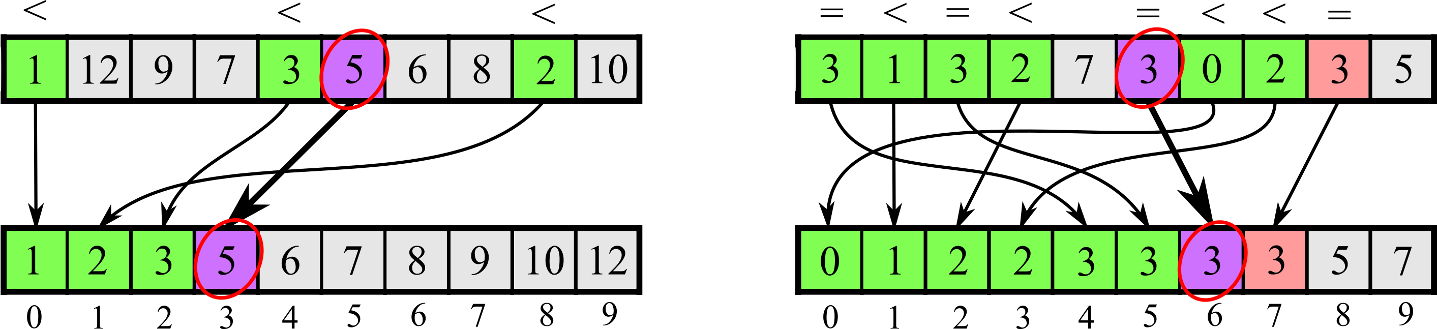
If equal elements are possible in the input array, then counting algorithm becomes more complicated. Let's try to make our sorting algorithm stable. Then the final position of element A[i] = X is equal to the number of elements less than X plus the number of elements equal to X located to the left of position i. It means that in addition to less elements, we also have to count number of equal elements, although only in about half of the array. This additional computation is inevitable, unless you are absolutely sure the input array has no duplicates.
The simple implementation of the suggested algorithm looks like this:
for (size_t i = 0; i < Count; i++) {
    int elem = inKeys[i];
    size_t cnt = 0;
    for (size_t j = 0; j < Count; j++)
        cnt += (inKeys[j] < elem);
    for (size_t j = 0; j < i; j++)
        cnt += (inKeys[j] == elem);
    dstKeys[cnt] = elem;
}
How should this sorting algorithm be called? I have never seen anything like this before. However, while looking for Green's sorting network at Morwenn's repository, I stumbled upon a page which contains an interesting link at the very end. It points to the so-called "Exact sort", which is exactly what I described just above. I don't like this name, because it gives too much attention to the very last step of the algorithm (i.e. moving elements to their places). In my opinion, the element-counting mechanic is the much more important part of the algorithm, which will be evident in the next section. That's why I prefer to call it "position-counting sort" ("counting sort" is already taken).
Let's recall the sacred four points. The algorithm is very simple in its core. It has no branches if fully unrolled (recall: array size is small and compile-time constaint). Note that the comparison does not generate a branch in x86. Unrolling this code is not recommended, even without unrolling branches should be well-predicted. As for data dependencies: outer iterations are completely independent, the inner loops behave like the reduce algorithm, so their iterations can be made quite independent from each other too. Finally, the data access patterns are very simple: inner loops access all elements sequentally (order does not even matter). This means that we can attempt to vectorize this algorithm.
Vectorization
As just noted, data dependencies are rather weak across iterations of both loops. So it makes sense to vectorize both by iterations of inner and outer loops. Vectorization of inner iterations should produce something like:
__m128i cnt = _mm_setzero_si128();
for (size_t j = 0; j < Count; j += 4) {
    __m128i data = _mm_load_si128((__m128i*)&inKeys[j]);
    cnt = _mm_sub_epi32(cnt, _mm_cmplt_epi32(data, elem_x4));
}
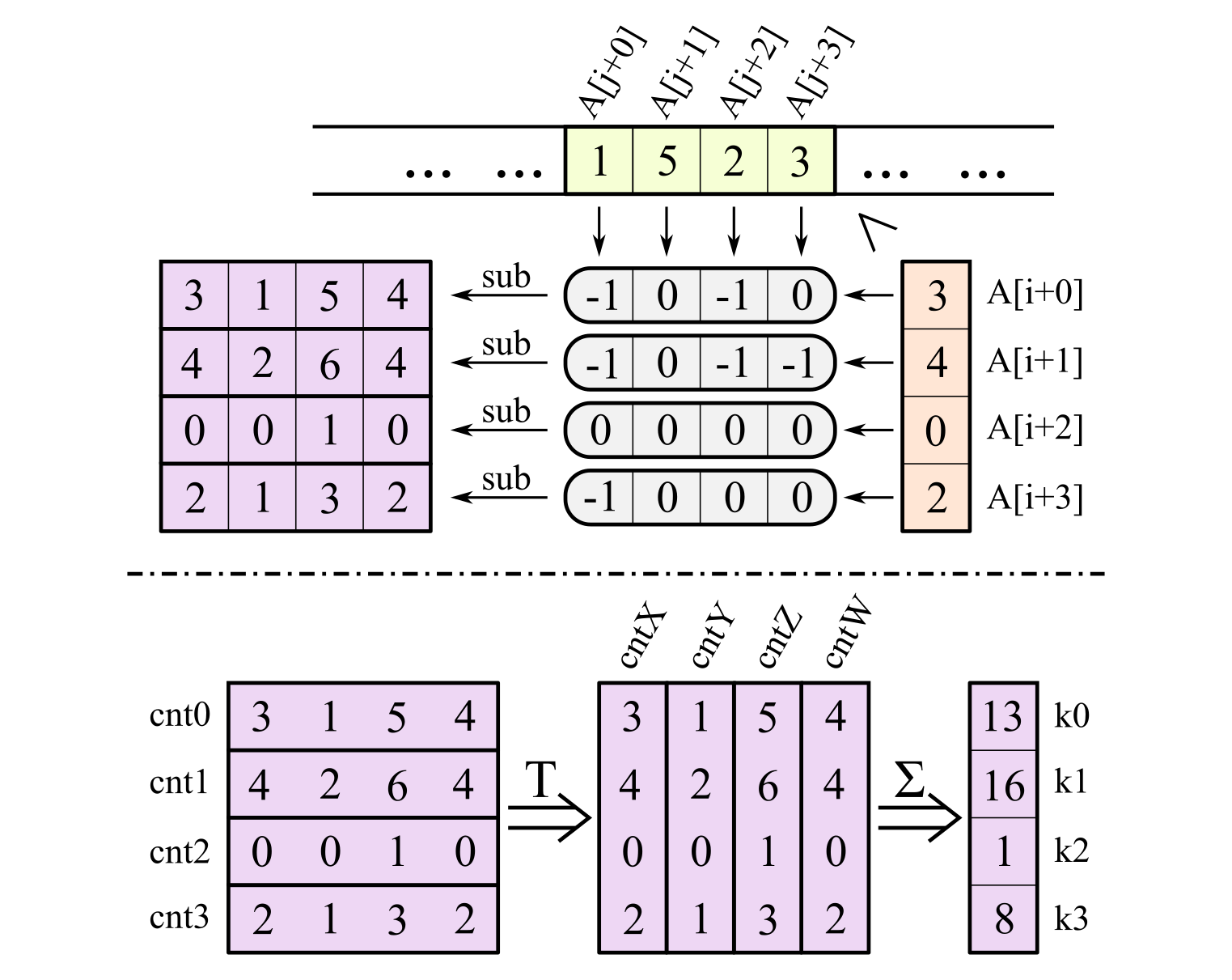
At the end, horizontal sum of cnt register has to be computed to obtain the sought-for final position of the considered element. In order to reduce number of loads, make horizontal sum faster, and in general reduce the overhead of loops, we can also process the elements to be moved in packs of four. So in the outer loop we load four elements at once too.
Here is the plan (bottom half shows horizontal sum at the end):
The code starts by iterating over the elements to be moved:
for (size_t i = 0; i < Count; i += 4) {
Here is the body of the outer loop:
//load four elements (to be moved into their locations)
__m128i reg = _mm_load_si128((__m128i*)&inKeys[i]);
//prepare a register with each value broadcasted
__m128i reg0 = _mm_shuffle_epi32(reg, SHUF(0, 0, 0, 0));
__m128i reg1 = _mm_shuffle_epi32(reg, SHUF(1, 1, 1, 1));
__m128i reg2 = _mm_shuffle_epi32(reg, SHUF(2, 2, 2, 2));
__m128i reg3 = _mm_shuffle_epi32(reg, SHUF(3, 3, 3, 3));

//init one register with counters per each element considered
__m128i cnt0 = _mm_setzero_si128();
__m128i cnt1 = _mm_setzero_si128();
__m128i cnt2 = _mm_setzero_si128();
__m128i cnt3 = _mm_setzero_si128();
for (size_t j = 0; j < Count; j += 4) {
    __m128i data = _mm_load_si128((__m128i*)&inKeys[j]);
    //update counters for all four elements of *reg*
    cnt0 = _mm_sub_epi32(cnt0, _mm_cmplt_epi32(data, reg0));
    cnt1 = _mm_sub_epi32(cnt1, _mm_cmplt_epi32(data, reg1));
    cnt2 = _mm_sub_epi32(cnt2, _mm_cmplt_epi32(data, reg2));
    cnt3 = _mm_sub_epi32(cnt3, _mm_cmplt_epi32(data, reg3));
}
Now we need to take equal elements into account. They are processed in very similar way, but only elements to the left of i are compared:
for (size_t j = 0; j < i; j += 4) {
    __m128i data = _mm_load_si128((__m128i*)&inKeys[j]);
    cnt0 = _mm_sub_epi32(cnt0, _mm_cmpeq_epi32(data, reg0));
    cnt1 = _mm_sub_epi32(cnt1, _mm_cmpeq_epi32(data, reg1));
    cnt2 = _mm_sub_epi32(cnt2, _mm_cmpeq_epi32(data, reg2));
    cnt3 = _mm_sub_epi32(cnt3, _mm_cmpeq_epi32(data, reg3));
}
Finally, there may be equal elements across elements i, i+1, i+2, i+3. We need to compare all elements in reg with each other, while carefully masking out the comparisons where operands go in wrong order:
//cnt0 = _mm_sub_epi32(cnt0, _mm_and_si128(_mm_cmplt_epi32(reg, reg0), _mm_setr_epi32( 0,  0,  0,  0)));
cnt1 = _mm_sub_epi32(cnt1, _mm_and_si128(_mm_cmpeq_epi32(reg, reg1), _mm_setr_epi32(-1,  0,  0,  0)));
cnt2 = _mm_sub_epi32(cnt2, _mm_and_si128(_mm_cmpeq_epi32(reg, reg2), _mm_setr_epi32(-1, -1,  0,  0)));
cnt3 = _mm_sub_epi32(cnt3, _mm_and_si128(_mm_cmpeq_epi32(reg, reg3), _mm_setr_epi32(-1, -1, -1,  0)));
Now all counts are gathered in XMM registers, and we have to calculate horizontal sum of each register. Since there are four of them, it makes sense to fully transpose them and then do a simple vertical sum:
//4x4 matrix transpose in SSE
__m128i c01L = _mm_unpacklo_epi32(cnt0, cnt1);
__m128i c01H = _mm_unpackhi_epi32(cnt0, cnt1);
__m128i c23L = _mm_unpacklo_epi32(cnt2, cnt3);
__m128i c23H = _mm_unpackhi_epi32(cnt2, cnt3);
__m128i cntX = _mm_unpacklo_epi64(c01L, c23L);
__m128i cntY = _mm_unpackhi_epi64(c01L, c23L);
__m128i cntZ = _mm_unpacklo_epi64(c01H, c23H);
__m128i cntW = _mm_unpackhi_epi64(c01H, c23H);
//obtain four resulting counts
__m128i cnt = _mm_add_epi32(_mm_add_epi32(cntX, cntY), _mm_add_epi32(cntZ, cntW));
Now we have final locations of all the four considered elements. We need only to extract them and move the elements to their places:
unsigned k0 = _mm_cvtsi128_si32(cnt   );
unsigned k1 = _mm_extract_epi32(cnt, 1);
unsigned k2 = _mm_extract_epi32(cnt, 2);
unsigned k3 = _mm_extract_epi32(cnt, 3);
dstKeys[k0] = inKeys[i+0];
dstKeys[k1] = inKeys[i+1];
dstKeys[k2] = inKeys[i+2];
dstKeys[k3] = inKeys[i+3];
That's all!
Comparison
Below you can see a barchart with performance comparison of all major implementations (on Ryzen 5 1600 with MSVC 2013 x64). Text label above each bar in format "1 / X" means than that the corresponding sort implementation takes X nanoseconds per call on average. In other words, its throughput is (1/X) sorts per nanosecond. The height of each bar is set as its throughput divided by throughput of std::sort (higher = faster).
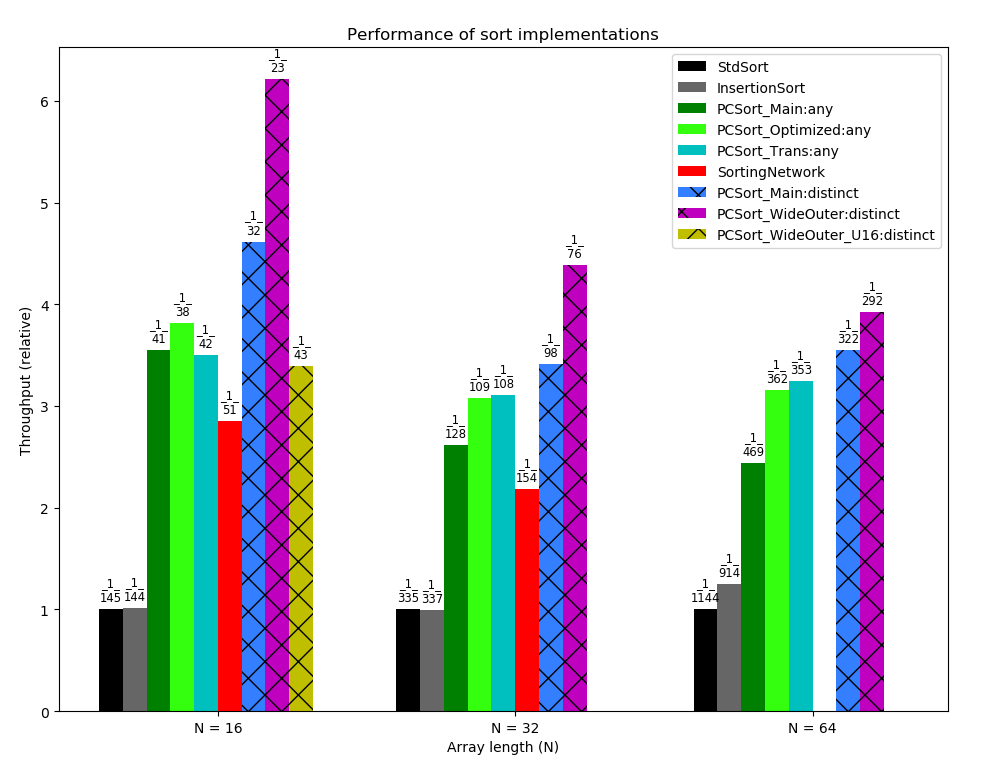
For instance, implementation PCSort_Main for N = 16 (dark green bar on the left) takes 41 nanoseconds per call, i.e. processes (1/41) calls per nanosecond. It is about 3.5 times faster than std::sort implementation.
The dashed bars correspond to implementations which work properly only on input arrays with all elements distinct.
Here is the explanation of different implementations:
- SortingNetwork: branchless sorting networks. For N = 16 it is Green's network of size 6 (as described above), for N = 32 it is something built on top of it (taken from here).
- PCSort_Main: the standard vectorized implementation of position-counting sort, exactly as described above.
- PCSort_Optimized: combines counting less elements and equal elements to the left of considered position into counting less-or-equal elements. This optimization allows to process each element of array only once per outer iteration (while in PCSort_Main the elements to the left are processed twice).
- PCSort_Trans: somewhat transposed implementation. A local array of N counters is created. The outer loop goes through the elements to compare with. The inner loop goes through the elements for which the final location is to be computed. During each outer loop, we have to pass through the array of counters and increase some of them. Note that optimization from PCSort_Optimized is already applied: each element is processed once per outer iteration.
- PCSort_WideOuter: this implementation uses wider vectorization in the outer loop compared to PCSort_Main, it computes final location for 16 elements during one outer iteration. In the inner loop elements are loaded in packs of four, and each element is broadcasted to the whole register to make comparison. This implementation works only for distinct elements: supporting equal elements in it is a major pain.
- PCSort_WideOuter: same as PCSort_WideOuter, but all loops are fully unrolled (works only for N = 16). To my surprise, it works slower than the version with loops.
According to the data, the standard position-counting sort (PCSort_Main) is 20-25% faster than sorting network for N = 16 and N = 32. The optimized implementations are even better for larger N (+17% for N = 32, and +30% for N = 64). If you are sure that all elements are surely distinct, you can get additional +30% performance boost. It is very important to note that the results differ a lot depending on compiler. 64-bit MSVC turned out to be the best compiler for position-counting sort, while network sort is much faster on 64-bit GCC (details in table below).
Below you can see performance plotted by N increasing. For each N and each method, the ratio of its speed to speed of std::sort is shown. For example, PCSort_Main is 3.5 times faster than std::sort for N = 16.
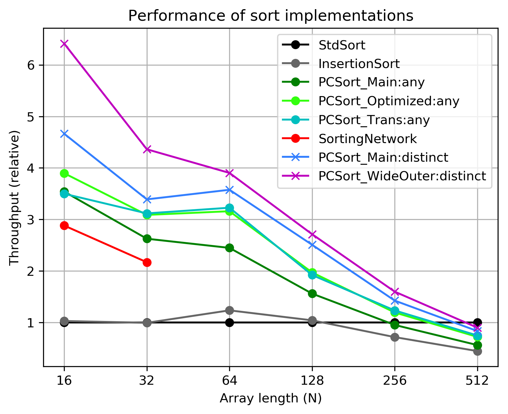
As you see, the proposed sorting method is always faster than insertion sort, and the std::sort implementation catches up with proposed method only for N = 256 (or a bit later for optimized/distinct-only versions).
I also mesured performance across several compilers and CPUs. The difference between compilers is surprisingly noticeable! Here is the full table:
| Platform | PC_Main | PC_Opt | Network | Insertion |
|---|---|---|---|---|
| Ryzen5 + VC2013 x64 | 127.8 | 108.7 | 153.5 | 334.7 |
| Ryzen5 + VC2013 x32 | 154.5 | 128.7 | 174.5 | 341.4 |
| Ryzen5 + GCC7 x64 (VM) | 119.4 | 127.3 | 100.8 | 347.4 |
| Ryzen5 + GCC5 x64 (VM) | 120.0 | 118.6 | 104.0 | 350.3 |
| Ryzen5 + GCC7 x32 (VM) | 140.4 | 118.7 | 154.7 | 430.7 |
| Ryzen5 + GCC5 x32 (VM) | 139.9 | 126.4 | 150.6 | 427.0 |
| Ryzen5 + TDM GCC5 x32 | 137.3 | 123.0 | 145.0 | 356.7 |
| i3-5005U + VC2017 x64 | 293.7 | 240.3 | 324.2 | 644.7 |
| i3-5005U + VC2017 x32 | 272.8 | 213.6 | 392.0 | 651.4 |
| i3-5005U + VC2013 x32 | 282.3 | 224.1 | 387.2 | 670.4 |
| i3-5005U + VC2015 x32 | 276.6 | 213.6 | 392.0 | 649.5 |
The list of CPUs used:
- Ryzen5: Ryzen 5 1600, 3.2 GHz
- i3-5005U: Intel i3-5005U, 2.0 GHz (Broadwell)
The list of compilers used:
- VC20xx: Microsoft Visual C++ of year 20xx (compiled with
cl.exewith/O2parameter). - GCC7: GCC 7.1.0 inside VirtualBox VM with Ubuntu (with
-O3 -msse4). - GCC5: GCC 5.4.0 inside VirtualBox VM with Ubuntu (with
-O3 -msse4). - TDM GCC5: TDM GCC 5.1.0 on Windows (with
-O3 -msse4).
As you see, 64-bit GCC manages to get 1.5 times faster performance from the sorting network. I suppose it succeeds in fitting everything into registers, while 32-bit GCC and MSVC cannot avoid register stalls. The position-counting sort also benefits from 64-bit case, most likely also due to having more XMM registers available.
Discussion
In practice, sorting only keys is rarely enough. In most cases each element consists of a key and an attached value, and an element must be moved as a whole during sort. There are two ways to store array of elements: having single array of key-value pairs (array-of-structures, AoS) and having two separate arrays, one with keys and the other one with values (structure-of-arrays, SoA).
It is very easy to extend the proposed algorithm to process keys with attached values, given that elements are stored in SoA layout, i.e. values are stored in a separate array. Since the vectorized part determines the final position (index) of every element, it is enough to send the values to same positions as their keys:
unsigned k0 = _mm_cvtsi128_si32(cnt   );
unsigned k1 = _mm_extract_epi32(cnt, 1);
unsigned k2 = _mm_extract_epi32(cnt, 2);
unsigned k3 = _mm_extract_epi32(cnt, 3);
dstKeys[k0] = inKeys[i+0];
dstKeys[k1] = inKeys[i+1];
dstKeys[k2] = inKeys[i+2];
dstKeys[k3] = inKeys[i+3];
//add this code to support values array:
dstVals[k0] = inVals[i+0];
dstVals[k1] = inVals[i+1];
dstVals[k2] = inVals[i+2];
dstVals[k3] = inVals[i+3];
No computations are added for values at all! Only a minimal amount of additional time is spent for moving every value directly to its final location. It takes O(N) time, which is dominated by O(N^2) part for counting positions. Although the keys are restricted to be 32-bit integers (32-bit floats can be supported the same way), the values can be of any type.
As for performance measurements, adding support for 32-bit values increases time per one sort for PCSort_Main:
- from 41 ns to 47.7 ns (+16.3%) for N = 16
- from 127.8 ns to 136.4 ns (+6.7%) for N = 32)
- from 465.4 to 486.4 ns (+4.5%) for N = 64.
Now compare it with sorting networks. Supporting values in a separate array (SoA) is more expensive: two additional CMOV operations must be added per one comparator (for swapping values conditionally). And it only works as long as the values are simple enough to be CMOV-ed. If the values are 32-bit, then it is much easier to work with array-of-structures layout. Store value first, key then, and treat each key-value pair as 64-bit integer. Compare them as 64-bit integers and CMOV them as such, and you'll get values support for free on 64-bit platform.
Compiler issue
I stumbled against a tiny compiler inefficiency. Visual C++ 64-bit compiler (and I guess other compilers too) generates unnecessary instruction for _mm_extract_epi32 intrinsic. Look at the assembly code generated by compiler for extracting single position and moving a key to its final location:
; 113  :  unsigned k2 = _mm_extract_epi32(cnt, 2);
; 117  :  dstKeys[k2] = inKeys[i+2];

;load inKeys[i+2] to eax:
mov     eax, DWORD PTR [rdx-16]
;extract k2 to ecx:
pextrd  ecx, xmm2, 2
;zero-fill upper half of ecx
mov     ecx, ecx
;store eax to dstKeys[k2]:
mov     DWORD PTR [r8+rcx*4], eax
For the first glance, the third instruction seems to do nothing. However, it was specifically inserted by compiler here, in order to clear the upper 32 bits of rcx register. What compiler does not know is that pextrd instruction already clears the upper 32 bits of 64-bit destination register, so the instruction is excessive.
The performance impact is most likely minimal, but it is still strange to see such things. The same issue happens for mm_movemask* intrinsics, see this question.
The code
As usual, all the materials and all the C++ code is available in position-counting-sort repo on GitHub.
Conclusion
The position-counting sorting algorithm is rather unknown, although it yields performance comparable to that of optimal sorting networks (which are well-known for their speed). It works in plain O(N^2) time, while sorting networks have to do somewhere between O(N log N) and O(N log^2 N) work. Having worse asymptotic complexity, it manages to be so fast only because it is vectorized very efficiently. So it can serve as a good alternative for sorting networks in some cases.